Importing the EEG/ERP data

Importing the data

Before you can go into the analysis of your data, you have to import all the EEG/ERP data and specify the design of the experiment. Make sure you have all your EEG/ERP data organized as follows:

• All data (i.e. all subjects and all conditions) are in the same subdirectory. Optimally, this subdirectory contains only the data that you want to import nothing else.
• For each subject and condition, there is an ASCII text file with the data. Each line of this file contains the measurements of all channels at one moment in time, each column in the file contains all moments of time of one channel. The program used the Matlab function 'load' to read the file. In case of trouble, look up Matlab's documentation on the function 'load'. Filenames should not contain spaces. As a decimal symbol, the "." is expected. No channel labels can be in the text files.
• All files of a single subject should have a common part in the name that uniquely identifies the subject.
• All files of a single condition should have a common part in the name that uniquely identifies the condition.
• All files have the same amount of channels and time-points, and the channels are always in the same order.
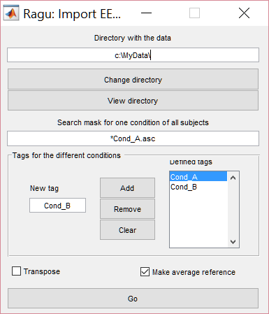
• Once you have organized the data as described above, you can proceed to import the data. In the dialog that opens when you click the Data->Import menu item, you have to set the necessary parameters. Typically, you work yourself thru the dialog from the top to the bottom. This contains the following
  • The subdirectory where all the data is located. Use the 'Change directory' button to navigate there. You can have a look at the content of the directory by clicking the 'View directory' button.
  • The search mask. Enter a string with Windows / OSX-wildcards in it that finds the files of exactly one single condition for all subjects. It does not matter which condition this is here. To illustrate this, lets assume you have data from 5 subjects, and 3 conditions. The data of subject 1 condition A is in a file called 'Sub1_Cond_A.asc', condition B of the same subject is in file 'Sub1_Cond_B.asc' condition B of subject 2 is in a file called 'Sub2_Cond_A.asc', and so on. A wildcard that identify the files of all subjects for one condition would for example be '*Cond_A.asc', or '*Cond_B.asc'. The tool is based on Matlab's 'dir' command, so check their documentation in case you run into problems or have further questions.
  • Tags for the different conditions. Enter the part of the filenames that uniquely identifies a single condition in the field New Tag' and press 'Add'. In the above example, this would e.g. be 'Cond_A'. Repeat until all conditions that you want to import are listed. In the above example, we'd have to add 'Cond_A', 'Cond_B' and 'Cond_C.
  • All data is recomputed against average reference by default. If you don't want this, uncheck the average reference checkbox. This applies namely to the case where you want to analyze non-negative power data.
  • You also have the options to transpose your data if your datafiles are channel x time  instead of time x channel matrices.
• Click Go. Based on the information that you have provided, the program is now able to construct all the filenames it can expect and load these files.
• You get a feedback on the dimensions of the entire set of data loaded. Make sure this corresponds to what you expected.

 When you have successfully imported the ERP data, you are directly taken to the dialogs that specify the remaining parameters of the data, i.e. your montage, and the sampling parameters.

Defining the montage

If you're not automatically arriving here, this procedure can be reached under Data->Montage. Here, you can (optionally) define the montage of your data, which will later allow you to better visualize the results. When you work with Analyzer and Matlab, you can simply save the Channel structure to a Matlab file and load this file as your montage. This is the procedure:

• Open one of your ERPs in the Analyzer
• In the Analyzer, start the Matlab transformation with the Command window shown and exporting all channels
• In the Matlab command window, type
  • Channel = Properties.Channels;
  • save MyFullOutfilepath.mat Channel
• return to the Analyzer, and close the Matlab window there.
• You can directly load the resulting Matlab file as the Montage

Alternatively, you can load a text file with the xyz coordinates of the electrodes. (x<0 is left x > 0 is right, y>0 is anterior, y < 0 is posterior), z > 0 is superior, coordinates should be on a sphere with radius 1 or use one of the standard sLORETA or CarTool electrode coordinate files. A sample file for download and editing is available here.

 Defining the sampling interval and latency of the first sample

Use the Data->Data Properties menu item to specify the sampling interval (time / frequency interval between adjacent points on the x-axis), sampling units and the X onset to get proper axes in your displays. Onset is defined as the latency of the first time-point of your data in reference to zero on the x-axis. Thus, if you have a 100ms pre-stimulus period, set the time onset to -100.